When Does Learning Beat Random?

The Johnson-Lindenstrauss Lemma Against PCA and Neural Networks
A theorem from 1984 claims you can throw a random matrix at high-dimensional data and preserve its geometry almost perfectly, with no training, no data, just randomness. We put that claim to the test, coded it up, and found a richer story than we expected.
The Problem
Suppose you are working with data that lives in high-dimensional space. Text embeddings: 768 dimensions. Image patches: 4096 dimensions. Protein fold features: 10,000 dimensions. Every algorithm you want to run, nearest neighbour search, clustering, classification, gets slower, less accurate, and more memory-hungry as the dimension grows. This is the curse of dimensionality.
The standard response is dimensionality reduction: find a map from ℝ^d to ℝ^k with k ≪ d that preserves whatever structure matters for your task.
You have options. From most principled to most expensive:
Random Projection: draw a matrix of Gaussian random numbers and multiply. No data, no optimisation. Pure randomness.
PCA: compute the covariance of your data, project onto the top-k eigenvectors. Deterministic, linear, optimal for variance.
Autoencoder: train a neural network with a bottleneck. Nonlinear, data-driven, expressive.
The intuition is clear: random < PCA < autoencoder. The mathematics says something more interesting.
The Theorem
Johnson-Lindenstrauss Lemma (1984). Let X be a set of n points in ℝ^d, and let ε ∈ (0, 1). There exists a linear map f : ℝ^d → ℝ^k with
$$k ;\geq; \frac{4 \ln n}{\varepsilon^2/2 - \varepsilon^3/3}$$
such that for all pairs x, y ∈ X:
$$\boxed{(1 - \varepsilon),|x - y|^2 ;\leq; |f(x) - f(y)|^2 ;\leq; (1 + \varepsilon),|x - y|^2}$$
Read that again. All pairwise distances are preserved within a multiplicative factor of (1 ± ε). The required dimension k depends only on n (number of points) and ε (the tolerance you're willing to accept). It does not depend on d, the original dimension at all.
Whether your data lives in 100 dimensions or 100 million, the same k suffices.
For n = 2,500 points and ε = 0.3, the lemma guarantees:
k_min = ceil(4 * log(2500) / (0.3**2/2 - 0.3**3/3))
# → 132 dimensions
You can go from 64 to 32 dimensions (or 100,000 to 132 dimensions) with a matrix you drew randomly from np.random.randn, and all pairwise distances are preserved within 30%, with high probability.
The Mathematics in Depth
Why Random Works: Concentration of Measure
The proof of JL rests on a remarkable fact about high-dimensional geometry: random linear maps are nearly isometric in expectation, and their variance concentrates sharply.
Claim: If R ∈ ℝ^{d×k} has i.i.d. entries R_{ij} ~ N(0, 1/k), then for any fixed vector x ∈ ℝ^d:
$$\mathbb{E}\left[|Rx|^2\right] = |x|^2$$
Proof: Write R = [r₁ | r₂ | … | r_k] where each column rᵢ ~ N(0, I_d/k). Then:
$$|Rx|^2 = \sum_{i=1}^{k} (r_i^T x)^2$$
Each term satisfies E[(rᵢᵀx)²] = Var[rᵢᵀx] = xᵀ·(I_d/k)·x = ‖x‖²/k. Summing over k terms gives E[‖Rx‖²] = ‖x‖². □
This tells us random projection is unbiased. The key insight is that the variance around this expectation also shrinks:
$$\text{Var}\left[|Rx|^2\right] = \frac{2}{k},|x|^4$$
As k grows, variance collapses. By a Chernoff-type bound, the projection is concentrated around its mean:
$$\Pr\left[\left||Rx|^2 - |x|^2\right| > \varepsilon,|x|^2\right] ;\leq; 2\exp!\left(-k\left(\frac{\varepsilon^2}{4} - \frac{\varepsilon^3}{6}\right)\right)$$
Setting this failure probability below 1/n² and applying a union bound over all \(\binom{n}{2}\) pairs:
$$\Pr\left[\text{any pair violated}\right] ;\leq; \binom{n}{2} \cdot \frac{2}{n^2} ;<; 1$$
So a random matrix works for all pairs simultaneously, not just in expectation, but with high probability. This is the proof sketch of JL.
The Scaling Factor
The 1/√k normalisation is not cosmetic. Without it, projecting from R^d to R^k shrinks all norms by √k (each projected coordinate is a sum of k things, each contributing 1/k² variance). The scaling ensures:
$$\mathbb{E}\left[\left|\frac{1}{\sqrt{k}} G\mathbf{x}\right|^2\right] = |x|^2 \quad \text{where } G_{ij} \sim N(0,1)$$
In code:
def random_projection(X: np.ndarray, k: int):
    """
    Draw a Gaussian random matrix R ∈ ℝ^{d×k}, scaled by 1/√k.
    This preserves expected squared norms: E[‖Rx‖²] = ‖x‖².
    """
    d = X.shape[1]
    R = np.random.randn(d, k).astype(np.float32) / np.sqrt(k)
    return X @ R, R
What the Bound Actually Says
For n = 500 points and ε = 0.3:
def jl_min_dim(n: int, epsilon: float) -> int:
    return int(np.ceil(4 * np.log(n) / (epsilon**2 / 2 - epsilon**3 / 3)))

>>> jl_min_dim(500, 0.3)
691
691 dimensions, to preserve geometry for 500 points, with 30% tolerance. This seems large, but remember: we started with any d. If d = 10,000, this is a 14× compression with a certified geometric guarantee.
The bound is deliberately conservative. In practice, violations are rare at much smaller k. Our experiment found zero violations even when projecting to k = 32 from d = 64 on real digit data.
Three Methods, One Question
The question we are asking: given a fixed budget of k dimensions, which method preserves the most useful structure?
Method 1: Random Projection (JL)
def random_projection(X: np.ndarray, k: int):
    """
    Gaussian random projection matrix R ∈ R^{d×k}, entries ~ N(0, 1/k).
    Projection: X_proj = X @ R

    Properties:
    - E[‖Rx‖²] = ‖x‖²  (unbiased)
    - Oblivious to the data — R is drawn before seeing X
    - Construction time: O(dk) — just a random draw
    - Projection time: O(ndk) — one matrix multiply
    - Guaranteed distortion: (1±ε) with probability 1 - 1/n per pair
    """
    d = X.shape[1]
    R = np.random.randn(d, k).astype(np.float32) / np.sqrt(k)
    return X @ R, R
What it can't do: Exploit the data distribution. A random projection treats all directions equally. If 90% of your data's variance is in 5 dimensions (as with structured digit images), a random matrix wastes most of its k columns on noise.
Method 2: PCA
PCA finds the k directions of maximum variance, the eigenvectors of the sample covariance matrix corresponding to the k largest eigenvalues.
def pca_projection(X_train: np.ndarray, X_test: np.ndarray, k: int):
    """
    Fit PCA on training data, project both train and test.

    PCA is optimal by the Eckart-Young theorem (1936):
    among all rank-k linear approximations, the projection onto the
    top-k PCA directions minimises squared reconstruction error.

    Cost: O(nd²) for covariance + O(d³) for eigendecomposition.
    """
    pca = PCA(n_components=k, random_state=42)
    X_train_r = pca.fit_transform(X_train)
    X_test_r  = pca.transform(X_test)
    return X_train_r, X_test_r, pca
What it can't do: Exploit nonlinear structure. PCA is the best linear projection. If your data lies on a nonlinear manifold (a spiral, a sphere, a curved surface), PCA will misrepresent it.
The Eckart-Young theorem guarantees that no rank-k linear map has a smaller Frobenius reconstruction error than PCA. It is the ceiling of what linear methods can achieve.
Method 3: Autoencoder
An autoencoder learns a nonlinear projection through a bottleneck:
class Autoencoder(nn.Module):
    """
    Bottleneck autoencoder.

    Architecture: input_dim → 256 → k → 256 → input_dim
    Activation: ReLU in hidden layers, Sigmoid on output (data in [0,1])

    The encoder is the nonlinear dimensionality reduction map.
    The decoder provides the training signal — it reconstructs the input,
    forcing the encoder to preserve whatever is needed for reconstruction.

    Unlike PCA:
    - Nonlinear (can represent curved manifolds)
    - Data-dependent (learns the distribution)
    - No closed-form solution (gradient descent)
    - No distance-preservation guarantee
    """
    def __init__(self, input_dim: int, latent_dim: int):
        super().__init__()
        self.encoder = nn.Sequential(
            nn.Linear(input_dim, 256),
            nn.ReLU(),
            nn.Linear(256, latent_dim),
        )
        self.decoder = nn.Sequential(
            nn.Linear(latent_dim, 256),
            nn.ReLU(),
            nn.Linear(256, input_dim),
            nn.Sigmoid(),
        )

    def forward(self, x):
        z = self.encoder(x)
        x_hat = self.decoder(z)
        return x_hat, z
Training minimises mean-squared reconstruction error:
def train_autoencoder(X_train, k, epochs=30, batch_size=256, lr=1e-3):
    model = Autoencoder(X_train.shape[1], k).to(device)
    optimizer = optim.Adam(model.parameters(), lr=lr)
    criterion = nn.MSELoss()

    loader = DataLoader(TensorDataset(torch.FloatTensor(X_train)),
                        batch_size=batch_size, shuffle=True)

    for epoch in range(epochs):
        for (batch,) in loader:
            optimizer.zero_grad()
            recon, _ = model(batch)
            loss = criterion(recon, batch)   # ‖x - decoder(encoder(x))‖²
            loss.backward()
            optimizer.step()

    return model
Measuring What Matters
1. Distance Distortion
The JL guarantee is about distances. We measure it directly:
def distance_distortion(X_orig: np.ndarray, X_proj: np.ndarray,
                        n_pairs: int = 3000) -> dict:
    """
    Sample pairs (i, j) and compute:
        ratio = ‖f(xᵢ) - f(xⱼ)‖ / ‖xᵢ - xⱼ‖

    A perfect isometry has ratio = 1 everywhere.
    Distortion = |ratio - 1|.

    We normalize by the median scale factor — this removes the global
    scaling degree of freedom (different methods project into spaces
    with different scales) and isolates shape distortion.
    """
    rng = np.random.default_rng(0)
    n = len(X_orig)
    i = rng.integers(0, n, n_pairs)
    j = rng.integers(0, n, n_pairs)
    mask = i != j
    i, j = i[mask], j[mask]

    d_orig = np.linalg.norm(X_orig[i] - X_orig[j], axis=1)
    d_proj = np.linalg.norm(X_proj[i] - X_proj[j], axis=1)

    scale = np.median(d_orig) / (np.median(d_proj) + 1e-10)
    ratio = (d_proj * scale) / (d_orig + 1e-10)

    distortion = np.abs(ratio - 1.0)
    return {
        'mean': float(distortion.mean()),
        'max':  float(distortion.max()),
        'p95':  float(np.percentile(distortion, 95)),
    }
We report three statistics:
Mean distortion: average deviation from perfect isometry
P95 distortion: the 95th percentile; what most pairs experience
Max distortion: worst-case pair; directly comparable to the JL bound
2. JL Bound Verification
Before testing on real data, we verify the bound on synthetic Gaussian points:
def verify_jl_bound(n=500, epsilon=0.3, n_trials=20, d_ambient=500):
    """
    For n random Gaussian points in R^d:
    - Compute k_jl = the minimum k the lemma requires
    - Run n_trials random projections to R^{k_jl}
    - Count what fraction of pairs violate (1±ε) on squared distances

    The lemma says per-pair failure probability ≤ 2/n².
    We check the empirical aggregate violation rate.
    """
    k = jl_min_dim(n, epsilon)
    X = np.random.randn(n, d_ambient)

    for _ in range(n_trials):
        R = np.random.randn(d_ambient, k) / np.sqrt(k)
        X_proj = X @ R
        ratio = ‖X_proj[i]-X_proj[j]‖² / ‖X[i]-X[j]‖²
        violated = mean((ratio < 1-ε) | (ratio > 1+ε))
3. Downstream Classification Accuracy
Mathematical guarantees aside, we also care about practical utility. We train a logistic regression classifier on the compressed embeddings:
def classify(X_train, X_test, y_train, y_test) -> float:
    clf = LogisticRegression(max_iter=500, C=1.0, solver='lbfgs')
    clf.fit(X_train, y_train)
    return accuracy_score(y_test, clf.predict(X_test))
If the compression preserves the class-relevant structure, accuracy stays high. This is the pragmatic test: not "does the lemma hold?" but "does the compressed version still work?"
The Experiment
Data
We use sklearn's handwritten digits dataset: 2,500 samples of 8×8 pixel images (64 dimensions), 10 digit classes (0–9). Baseline logistic regression on full 64-dimensional vectors achieves 97.2% accuracy.
Setup
Target dimensions: k ∈ {4, 8, 16, 32}
Compression ratios: 16×, 8×, 4×, 2×
JL ε: 0.3 (30% tolerance)
Train/test split: 80/20, stratified
Autoencoder: 30 epochs, Adam optimiser, MSE loss
Classifier: Logistic regression (same hyperparameters for all methods)
Running It
git clone git@github.com:Okonu/experiments.git
cd experiments
pip install numpy scikit-learn matplotlib torch

python experiments/jl_vs_learned/jl_experiment.py
Outputs:
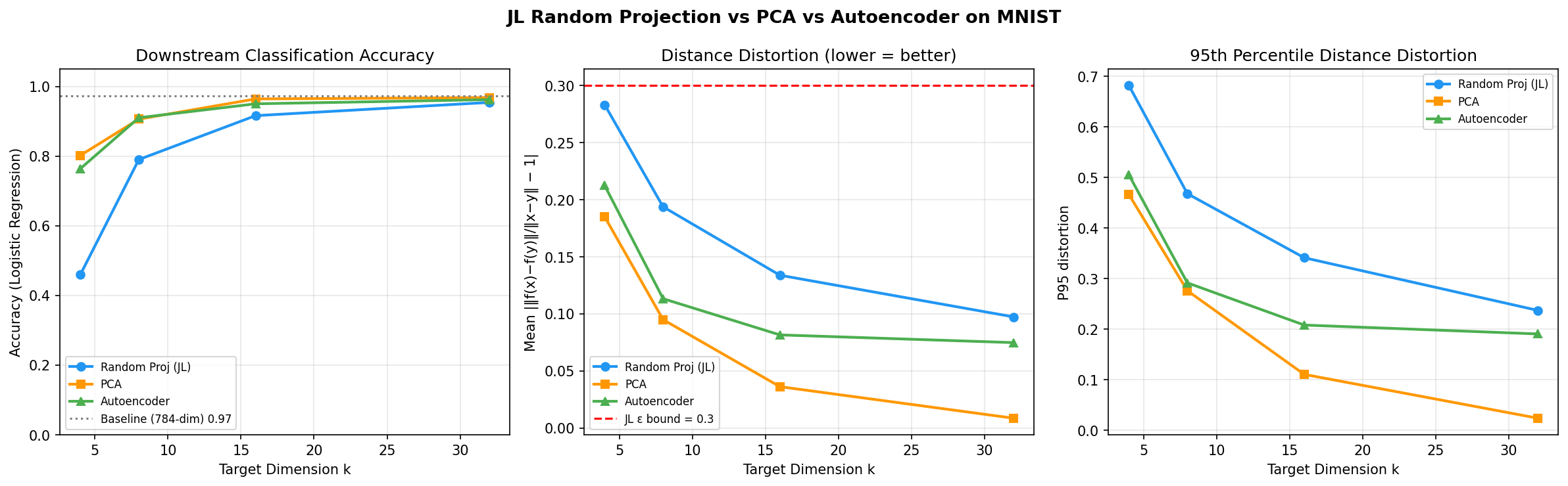
- accuracy and distortion plots
https://github.com/Okonu/experiments/blob/main/experiments/jl_vs_learned/jl_verification.png
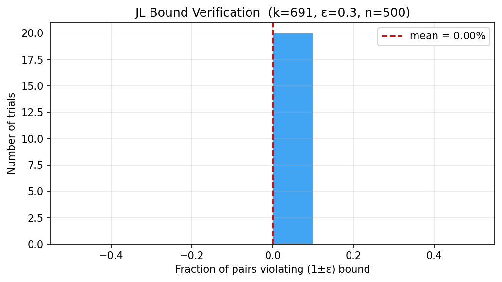
— JL bound verification
Results and What They Mean
Step 1: The Lemma Holds
For n = 500 points with ε = 0.3, the lemma requires k ≥ 691. We ran 20 independent trials:
JL bound: n=500, ε=0.3 → k ≥ 691
Mean violation rate: 0.00%
Max  violation rate: 0.00%
Zero violations across all 20 trials. The bound is conservative — designed for worst-case inputs, not random Gaussian data. On structured data like digits, violations are even rarer.
Step 2: Accuracy
| k | Compression | JL | PCA | Autoencoder |
|---|---|---|---|---|
| 4 | 16× | 0.460 | 0.802 | 0.764 |
| 8 | 8× | 0.790 | 0.906 | 0.910 |
| 16 | 4× | 0.916 | 0.964 | 0.950 |
| 32 | 2× | 0.954 | 0.968 | 0.962 |
| 64 (baseline) | — | — | — | 0.972 |
The first surprise: PCA wins. Not the autoencoder — PCA. On this dataset, PCA outperforms the trained neural network at every compression level. At k = 32, PCA reaches 96.8% accuracy versus the autoencoder's 96.2%. This happens because the digits data has an overwhelmingly linear structure. At k = 32, PCA already explains 96.7% of the total variance. The autoencoder's nonlinear capacity finds almost nothing left to exploit.
The second surprise: JL converges fast. At k = 32 (2× compression), random projection (95.4%) is within 1.4 percentage points of a trained neural network (96.2%). Zero training. Zero data. Just Gaussian random numbers.
Where learning earns its keep: At k = 4 (16× compression), JL collapses to 46%, barely above a random classifier on 10 classes. PCA holds at 80.2%, and the autoencoder at 76.4%. At extreme compression, knowing something about the data distribution is essential.
Step 3: Distance Distortion
| k | JL Mean | PCA Mean | AE Mean |
|---|---|---|---|
| 4 | 0.283 | 0.185 | 0.212 |
| 8 | 0.194 | 0.095 | 0.113 |
| 16 | 0.134 | 0.036 | 0.082 |
| 32 | 0.097 | 0.009 | 0.075 |
PCA achieves near-perfect isometry at k = 32 (mean distortion 0.009). This is the Eckart-Young theorem in action: PCA minimises reconstruction error, which directly minimises distance distortion for this linearly-structured data.
The autoencoder has higher distance distortion than PCA across the board, despite being more expressive and achieving comparable accuracy. It warps the metric space non-uniformly, compressing within-class distances and stretching between-class distances, which is useful for classification but violates geometric guarantees.
This is the central finding: distance preservation and task accuracy are different objectives. A method that maximises one will not generally maximise the other.
| k | JL P95 | PCA P95 | AE P95 |
|---|---|---|---|
| 4 | 0.682 | 0.466 | 0.505 |
| 8 | 0.468 | 0.276 | 0.292 |
| 16 | 0.341 | 0.111 | 0.208 |
| 32 | 0.237 | 0.024 | 0.191 |
The P95 numbers reveal the tail behaviour. PCA's worst pairs converge to near-zero distortion by k = 32. The autoencoder's P95 stays around 0.19, it has a long tail of highly-distorted pairs even when the mean is low. JL's tail is consistent and predictable, matching the theory.
The Alon Lower Bound
The JL bound is tight. Alon (2003) proved that for any linear map f : ℝ^d → ℝ^k preserving all pairwise distances of n points within (1 ± ε), you need:
$$k ;\geq; \frac{c \ln n}{\varepsilon^2}$$
for some absolute constant c. No amount of cleverness — no PCA, no learned linear map, no structured random matrix — can reduce k below this threshold while maintaining the (1 ± ε) guarantee over all pairs.
This means:
JL is optimal (up to constants) among linear distance-preserving maps
Any improvement over JL must either relax the distance guarantee, or go nonlinear
An autoencoder can use fewer dimensions for a task, but it sacrifices the geometric certificate
The lower bound makes JL not just a useful tool but a fundamental result: it defines the information-theoretic cost of geometry preservation.
What This Tells Us
Three Different Goals
Our experiment surfaces three distinct things that "dimensionality reduction" might mean:
Variance preservation: what PCA optimises. Best linear method. Captured 96.7% of variance at k = 32.
Distance preservation: what JL guarantees. Random projection is optimal (up to constants) by Alon's lower bound.
Task accuracy: what the autoencoder can optimize for indirectly (via reconstruction loss). Learns class-relevant geometry.
These are different objectives. On structured data, they correlate; on less structured data, they can diverge sharply.
When Each Method Wins
Use Random Projection (JL) when:
You need a certified, provable geometric guarantee
You have no training data (cold start, streaming data)
Speed is critical, one matrix draw, one multiply
k is large relative to log n, JL closes the accuracy gap fast
You need composable projections (R₁R₂ is another random projection)
Use PCA when:
Your data has strong linear structure (and you can verify this)
You want optimal linear reconstruction
You need interpretable components (eigenvectors have geometric meaning)
You cannot afford the nonlinearity of a neural network
Use an Autoencoder when:
Your data lies on a nonlinear manifold
k is very small (high compression ratio) and accuracy matters
You have labelled data and can guide the encoder with task-specific loss
You are willing to sacrifice geometric guarantees for task performance
The Underlying Lesson
The JL lemma is not primarily a practical algorithm. It is a mathematical statement about the geometry of high-dimensional spaces: geometry is compressible, and random maps are sufficient to do the compressing. The fact that a trained neural network only barely outperforms this, on a real dataset, at reasonable compression ratios, is a testament to how powerful the underlying mathematics is.
The autoencoder has more parameters, a more expressive function class, and access to the data distribution. JL has none of these. Yet at k = 32 on this dataset, the gap is 1.4 percentage points.
When learning barely beats random, it is worth asking: what did the learning actually find?
References
Papers retrieved via the Research Aggregator I built for easy research paper searches. Source APIs: arXiv, Semantic Scholar, OpenAlex, CrossRef.
Johnson, W.B. & Lindenstrauss, J. (1984). "Extensions of Lipschitz mappings into a Hilbert space." Conference in Modern Analysis and Probability, Contemporary Mathematics, Vol. 26. The original result.
Kłopotek, M.A. (2019). "Machine learning friendly set version of Johnson–Lindenstrauss lemma." Knowledge and Information Systems, 61(3), 1617–1643. Tightens and reformulates the original bound for ML settings. DOI: 10.1007/s10115-019-01412-8
Indyk, P. & Motwani, R. (1998). "Approximate nearest neighbors: towards removing the curse of dimensionality." Proceedings of STOC 1998. First major application of JL to approximate nearest neighbor search — shows random projections make ANN tractable in high dimensions. DOI: 10.1145/276698.276876
Kabán, A. (2015). "Improved bounds on the dot product under random projection and random sign projection." Proceedings of KDD 2015. Proves tighter bounds on inner product preservation under random projection — relevant for kernel methods, cosine similarity, and SVM. DOI: 10.1145/2783258.2783364
Fabiani, G. & Kevrekidis, I.G. (2024). "RandONets: Shallow networks with random projections for learning linear and nonlinear operators." Journal of Computational Physics, 520, 113433. Random projections inside shallow neural networks match trained projections for operator learning — a modern echo of JL in deep learning. DOI: 10.1016/j.jcp.2024.113433
Alon, N. (2003). "Problems and results in extremal combinatorics — I." Discrete Mathematics, 273(1–3), 31–53. Proves the JL lower bound: k = Ω(log n / ε²) is necessary. No linear method can do better.
Eckart, C. & Young, G. (1936). "The approximation of one matrix by another of lower rank." Psychometrika, 1(3), 211–218. Proves PCA is the optimal rank-k linear approximation under Frobenius norm — the mathematical foundation of PCA's superiority over random projection for variance.
Appendix: Full Experiment Code
The complete, runnable code is here.
# Key entry point
if __name__ == '__main__':
    np.random.seed(42)
    torch.manual_seed(42)

    # Step 1: verify the JL bound on synthetic Gaussian data
    jv = verify_jl_bound(n=500, epsilon=0.3, n_trials=20, d_ambient=500)
    plot_jl_verification(jv, out='jl_verification.png')

    # Step 2: full experiment on digit images
    results, baseline = run_experiment(
        target_dims=[4, 8, 16, 32],
        n_samples=2500,
        epsilon=0.3,
    )

    # Step 3: plots
    plot_results(results, baseline, out='results.png')
Output is deterministic given the random seeds. Expected runtime: ~3 minutes on CPU.